Table of Contents
- Interplanetary and Interlunar Transfer Calculator
- Overview
- Specifics
- Interstellar Transfer
- Brachistochrone Transfer (Epstein Drive)
- Propagation Delay Calculator
- Rendering the Orbits and Planet Positions
- Orbits and Planets
- System Updating
- Axial Tilts
- Displaying in 3D SBS Format
- Three.JS Graphics
- Shadows and Moon Occultations
- Ship Alignment
- Dynamic Texture Loading
Interplanetary and Interlunar Transfer Calculator
The system uses Gauss’s solution to Lambert’s problem to calculate valid trajectories for each transit time and planet position. This solution takes in two position vectors (of the planets) and the transit time between planets, and returns two velocity vectors of the ship at each planet position. It then finds the magnitude of the difference between the returned velocity vector and the planet’s own velocity vector, and then use the minimum change in velocity (minimum ΔV) trajectory as the best trajectory. It then calculates the orbital parameters based on the position and velocity vector. All courses are stored, and are then used to render the porkchop plot. The porkchop plot is a contour map of the characteristic energy required for the maneuvers, where red is worse and blue the best. The fissure in the center of the plot results from the calculator, as when the phase angle is close to pi, the resultant orbit is steeply inclined to the plane of the ecliptic, resulting in a large ΔV.
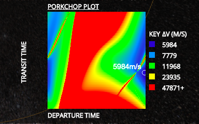
Porkchop Plot of an Earth-Mars Transit
The main transfer engine and attendant functions are about a thousand lines in total, excluding generalised vector manipulation and conversion functions. The program uses a system of timeout functions that ensures that the program does not freeze while it is calculating, and that it can have a loading screen.
Going into detail about the solution; the way the system iterates is it iterates through 200 positions for the starting time (going from zero to the synodic period), and 200 positions for the transit time, from 0.05 to 1.95 of the estimated transfer time. It finds the initial planet’s position at the start, and the final planet’s position at the end of the transfer, and their respective velocity vectors. A series of equations are then used, but one value cannot be found algebraically (the semi-latus rectum). The system uses a linear convergence algorithm, calculating the time associated with the value of the semi-latus rectum, and then refining. Initially a binary convergence algorithm was used, but it was unsuitable due to the graph’s gradient going from positive to negative (see below), and often produced invalid trajectories(binary requires one or the other to function). The correct p-value must be selected or the actual transfer time and the used transfer time differ, and this makes all subsequent calculations invalid. The system has a custom loading script while the computer runs all the calculations, as it needs to investigate 40,000 different transfer windows, and must execute an iterative convergence algorithm for each.
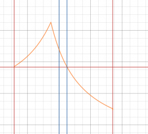
Graph of calculated transfer time with respect to semi-latus rectum
The required ΔV is found by the difference between the needed velocity vector and the planet’s velocity vector. For planets with a significant gravity well, a hyperbolic trajectory is determined, and the ΔV required to enter orbit is used instead, with the hyperbolic excess velocity being the difference between the needed velocity and the planet’s velocity (this is different due to the Oberth Effect). The parameters are then determined using the angular momentum of the ship to calculate the inclination and ascending node, and the semi-major axis from the magnitude of the velocity vector. The eccentricity is determined using a series of equations, using the cross product of the velocity and position vectors. The mean longitude at epoch used to be determined using a progressive binary convergence algorithm, which meant that it needed to calculate only log(3600) * 10 times, rather than 3600. However, this had a flaw in some occasional edge cases where it focused in on a spot that looked promising, but was actually not the right location. It has been replaced with one that uses the same process that it uses to find planetary locations in reverse, so that it reverse-derives the mean longitude at epoch instead of running hundreds of iterative calculations. This has the added advantage of being much faster, and so therefore not requiring a loading time for determining parameters of about the same length as the calculation.
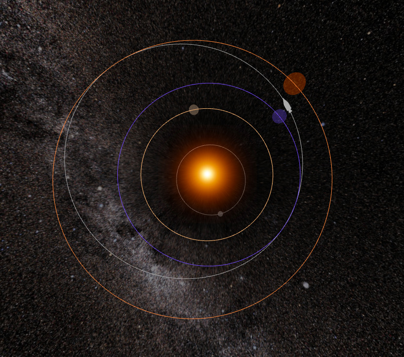
The final Earth-Mars transfer orbit
The system is more accurate than a simple Hohmann transfer orbit, as a Hohmann transfer assumes a phase angle of pi, no relative inclination, and no eccentricity in the orbits. The transfer calculator is completely dynamic, and function for even highly eccentric and inclined objects, such as some asteroids and comets.
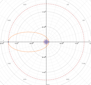
A hohmann transfer between two circular orbits
Interstellar Transfer Calculator
The interstellar transfer uses an accelerate – coast – deceleration profile. It takes in a constant proper (non-relativistic) acceleration from the spacecraft, which leads to decreasing rest acceleration due to relativity as the ship approaches the asymptote of the speed of light. It calculates both the time for an observer at Earth observing the spacecraft, and the time on the spacecraft itself. To calculate the ship time and displacement, it uses the formula relating acceleration and proper acceleration, and then integrating by either position or time.
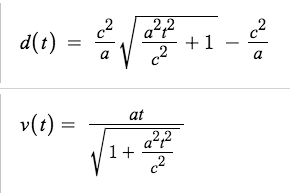
Expressions for relativistic distance and velocity as a function of proper time and a constant proper acceleration.
To calculate time aboard ship during acceleration and deceleration, the velocity expression is substituted into the time dilation expression and then integrated with respect to time. These expressions are then combined to calculate the maximum velocity, the total time aboard ship, and the total time at Earth. The right ascension and declination of the stars are used to show the ship travelling off in the correct direction, calculated through the same axial tilt method as above.
The ship actually compresses as described by Lorentzian length contraction, with the Lorentz factor being calculated from the velocity equation above. The ship increases in size as it departs the Sol System to ensure it is visible, so the length contraction means that the lengthwise size doesn’t grow as quickly as the others. The proportions are accurate at all times.
Brachistochrone Transfer (Epstein Drive)
To find the brachistochrone trajectory, the system estimates the approximate transfer time and iterates around that to find the best transfer. The trajectory itself is calculated by first determining the travel vector, and then determining the velocity component aligned with the travel vector. The ship decelerates to burn off any velocity in the incorrect direction, and then moves along the transfer line, with a starting velocity determined by what remains of the planet’s velocity. It then constantly accelerates, and then decelerates along the main transfer vector. It then uses the inverse of the process to neutralise velocity not aligned to the travel vector to match velocities with the destination planet.
Propagation Delay Calculator
To find the propagation delay between objects, the system subtracts the position vector of the central object from the position vector of the desired object. The magnitude of the resultant vector divided by the speed of light gives the delay for the desired object. The propagation delay is the minimum time (excluding relays and signal processing time) a signal takes to travel between planets, as it is limited through the speed of light and relativity.
Rendering the Orbits and Planet Positions
The orbital parameters for each planet are stored in JSON format. Each orbit is rendered as an ellipse, with the body’s orbital center (sun or planet) as one foci. For the graphics engine, they are considered as a number of separate points with a separation of 0.1 degrees between each point. The magnitude of the velocity is calculated at each point (using the vis-viva equation), and to find the velocity vector, it approximates that the tangent was in the same direction as the next point on the ellipse. The time between each point was calculated by dividing the magnitude of the distance vector by the magnitude of the velocity vector. It stores the sum of previous times next to each degree (with 0 being its location at the J2000 epoch), and then to find the position at a given time it takes the modulus of the current time and the orbital period, and then iterates through the list of orbital times until it finds the correct location (where the found time exceeds the orbital time). It then takes the two points that the planet must be between, and approximates that it moves at a constant velocity along the 0.1 degree segment to make it move more smoothly, rather than jumping between the increments
The system does this for all planets 100 times per second, and also moves the moons, moon orbital tracks and cameras relative to the parent planets at the same time so that the system moves everything smoothly without leaving anything behind. The system has been heavily optimised, and ensured that it stores the results of as many calculations as possible, so that it can still function without freezing or slowing down on small devices such as a laptop. All these calculations are done on startup, and they are then stored for use for the rest of the program. It also does not display the surfaces of planets unnecessarily, and does not display moons until the parent planet is centered. There are toggles to enable the smaller bodies and satellites, as they are not in the program by default to prevent excessive clutter.
Axial tilts complicate the calculations for moons, as the orbital parameters are measured from the planet’s equator, not the plane of the ecliptic like the rest of the program. The angular velocity is found using the inclination and longitude of the ascending node. It then takes the cross product of the z-vector and the planet’s axial tilt (the vector describes where the north pole points), and then find the angle between them with a dot product. The angular velocity vector is then rotated around the cross product by the angle found previously. The new orbital parameters (relative to the ecliptic), the longitude of the ascending node and inclination, are then calculated. The rendering process then proceeds as normal with the new parameters.
Three.JS Graphics
Shadows and Moon Occultations
Despite appearances, the sun is not actually the source of light. To create shadows correctly, a spotlight is placed at a position along a straight line from the planet to the sun, at 0.9 times the distance. It is then pointed at the planet, with a very wide angle to ensure it illuminates the moons. Shadows are handled separately than lighting, by a camera system. An orthographic shadow camera is used to mimic the sun’s effectively parallel rays after travelling a few AU. The shadow camera is pointed at the planet itself, so that moons are shadowed when passing behind and moons cast their own shadows upon the planet.
Ship Alignment
The ship is aligned by using a a series of quaternions. Each part of the ship is individually textured, and placed in a group for collective manipulation. By aligning the group to allow for the rotation of the ship, it can be rolled. By placing another group around that, and aligning it to the direction of travel, the ship can point in the correct direction.
Dynamic Texture Loading
The program already has a long loading sequence, but loading all the textures on startup (especially with a slow internet) would hake it a lot longer. The system automatically renders all planetary textures as spheres the same colour as the orbital track (this is what you see in the Low Res version). All surface textures are hidden upon rendering to save on computational power. Upon looking at a planetary surface, the program re-colours the model and places the map on it to texture it. A similar process happens for objects with models such as comets and small asteroids.